First day cover ·
Excel's Preview Lets One Cell Hold Lists and Arrays
Excel's preview feature lets a single cell hold lists, arrays and nested arrays. Here's what it solves, who can try it and what to watch for.
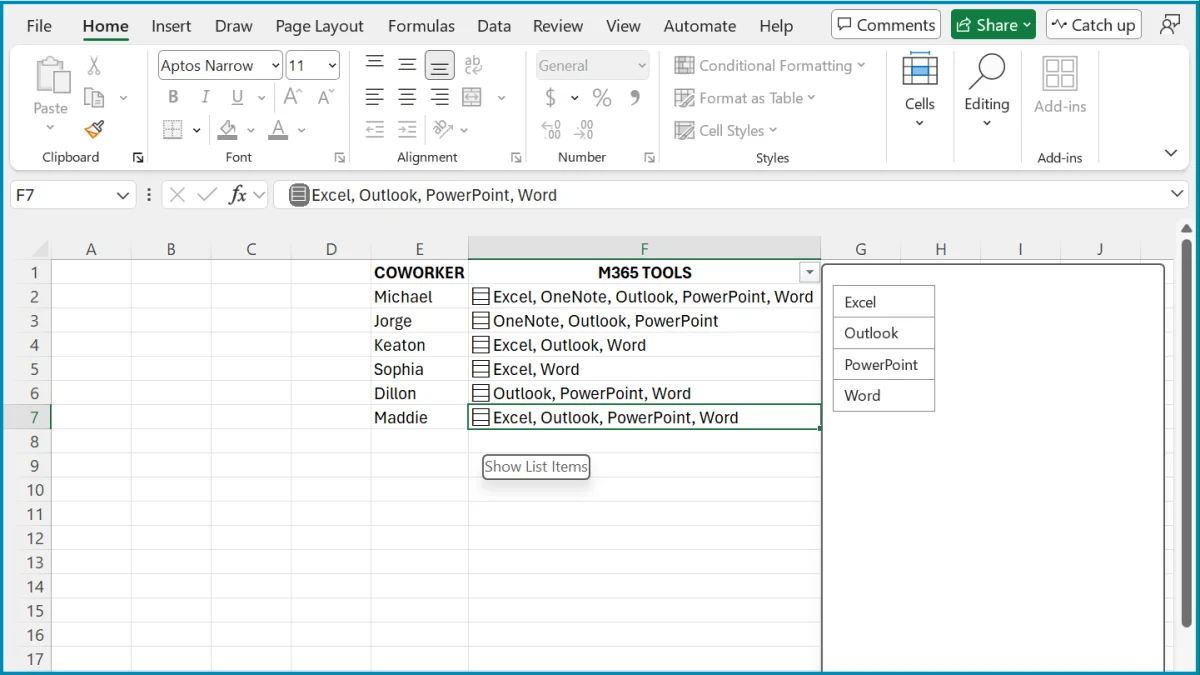
For as long as spreadsheets have existed, a cell has held one value. You can cram a few items into a cell with commas, and dynamic array formulas can spill results across neighbouring rows and columns, but the cell itself is still a single-item box. Excel's latest preview changes that. It lets one cell hold several structured values at once, and that shifts how you might lay out a sheet.
Three new structures
The preview adds three in-cell data types. The first is the list, which keeps a sequence of independent items in a single column. The difference from a comma-separated string matters: Excel treats each entry as its own element. A single list can mix text, numbers, dates and Boolean values, and each item keeps its native data type.
The second is the array, a grid of rows and columns sitting inside one cell. The third is the nested array, where formulas can generate arrays inside other arrays. That gives complex output a home inside one cell rather than forcing it across the worksheet grid.
Who can try it, and who has to wait
Right now the feature is limited to Excel for Windows and Mac, and only for members of the Microsoft 365 Insider program on the Beta Channel. Microsoft hasn't said when it will reach all Microsoft 365 subscribers. Perpetual licence versions such as Office 2021 and Office 2024 don't support it, and neither does Excel for the web. If you're on one of those, this is a feature to bookmark rather than plan around.
Where it earns its keep
The clearest case is multi-item categorising. Picture a team where each person is skilled in up to five Microsoft 365 apps, or sells across several product categories. The usual approach gives each app or category its own column. That works until the sheet also needs contact details, notes and status fields, and suddenly you're scrolling sideways through a wall of columns.
With an in-cell list, all of those skills sit in one column. The useful part is that Excel recognises each item individually, so the column's filter drop-down lets you pick one skill, or a combination of them, and see matching rows. You get the tidiness of one column without losing the ability to query each entry.
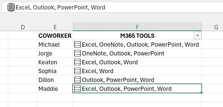
In-cell lists collapse what would otherwise be several columns into one.
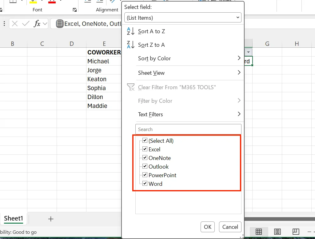
Because each item is recognised separately, the filter can work on individual entries.
Survey data is another natural fit. When respondents rate a set of questions on a numerical scale, you can store all of one person's answers in a single cell rather than dedicating a column to every question. Anyone who has built a sheet with dozens of question columns will recognise the appeal, especially when the rest of the sheet holds other per-person details.
The third use case is more technical and, to my mind, the most practical. Functions like TEXTSPLIT applied down a whole column normally try to spill their results sideways for every row at once. If anything sits in the way, you get a #SPILL! error. Packing each row's split output into a nested array keeps the result to one column, so nothing spills across the grid and the collision disappears.
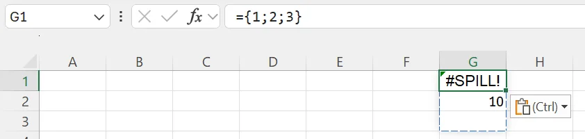
Here the array in G1 has nowhere to spill because G2 is already occupied.
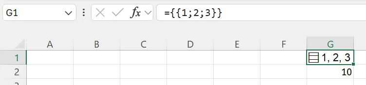
Wrapped in a nested array, the same output stays inside one cell and the error clears.
Creating and reading in-cell data
To make a list, select a cell and press Ctrl + J to open the in-cell list editor, or go to Insert > List on the ribbon. Type or paste items separated by commas or line breaks.
Arrays use curly braces. ={1;2;3} creates a standard array that spills across cells. Wrap it in a second set of braces, as in ={{1;2;3}}, and it stays in one cell. The same trick works on formulas: ={TEXTSPLIT(B3,, ", ")} places the whole result inside a 1×1 container and suppresses the spill. Nested arrays go one level further, such as ={{1,2,3};{4,5,6}}, which builds multiple rows and columns inside a single cell.
Referencing works differently. If a cell points directly at a cell holding a list or array, say =B6, Excel spills the internal contents into the grid. To pull out a specific element without spilling, use INDEX or the field access operators.
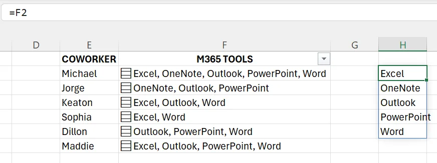
Entering =F2 in H2 pulls every item out of the in-cell list in F2.
The trade-offs
Packing data into cells makes it harder to see. A conventional grid shows everything at a glance, and in-cell structures make people click in to see the detail, which slows auditing. Memory use runs somewhat higher than for single values, and calculations can be slower. Nested arrays generally need Compatibility Version 3, which you set under Formulas > Calculation Options.
Compatibility is the bigger practical issue. A worksheet with these structures will show formula errors in older desktop, perpetual or unsupported versions, so tell your collaborators before you share the file. Legacy functions such as SUMIF, COUNTIF and VLOOKUP may not inspect values inside multi-value cells unless you wrap them or switch to modern alternatives like XLOOKUP or BYROW. The preview also adds four functions for array work: FLATTEN unpacks nested arrays into rows and columns, while HAS, HASANY and HASALL check whether particular values appear inside an array.
Microsoft warns that behaviour may change based on feedback from Insiders before general release, so treat any workbook built on these features as a work in progress for now. My read: the spill-error fix and the tidier multi-item columns are worth testing on a copy of a real sheet today, but I'd hold off on making them the backbone of a shared file until the feature reaches everyone and the compatibility picture settles.